1.समतल वक्रों की लम्बाईयां (Lengths of Plane Curves)-

• समतल वक्रों की लम्बाईयां (Lengths of Plane Curves) को चापकलन (Rectification) कहते हैं।समतल वक्रों की लम्बाईयां ज्ञात करने के लिए कई सूत्र प्रयोग में लिए जाते हैं।
• जैसे कार्तीय समीकरणों के लिए,कार्तीय समीकरण को प्राचलिक रूप में लिखकर, ध्रुवीय रूप में वक्र का समीकरण,पदिक समीकरण इत्यादि के लिए अलग-अलग सूत्रों का प्रयोग किया जाता है।ये सूत्र वक्र की आकृति पर निर्भर करते हैं।
• समतल वक्रों की लम्बाईयां(Lengths of Plane Curves) ज्ञात करने के लिए समाकलन के साथ-साथ अवकल गुणांक का प्रयोग किया जाता है।समतल वक्रों की लम्बाईयां(Lengths of Plane Curves) ज्ञात करने के लिए एक आर्टिकल पूर्व में भी पोस्ट किया हुआ है।अतः सूत्रों को जानने तथा थ्योरी हेतु उस आर्टिकल को भी देखना चाहिए।
  
• आपको यह जानकारी रोचक व ज्ञानवर्धक लगे तो अपने मित्रों के साथ इस गणित के आर्टिकल को शेयर करें।यदि आप इस वेबसाइट पर पहली बार आए हैं तो वेबसाइट को फॉलो करें और ईमेल सब्सक्रिप्शन को भी फॉलो करें।जिससे नए आर्टिकल का नोटिफिकेशन आपको मिल सके ।यदि आर्टिकल पसन्द आए तो अपने मित्रों के साथ शेयर और लाईक करें जिससे वे भी लाभ उठाए ।आपकी कोई समस्या हो या कोई सुझाव देना चाहते हैं तो कमेंट करके बताएं। इस आर्टिकल को पूरा पढ़ें।

Also  Read This Article:-Volume of Solids of Revolution

2.समतल वक्रों की लम्बाईयां के सूत्र (Lengths of Plane Curves Formulas)-

We know that Differential Calculus if s denotes the length of arc of the curve given by y=f(x) from a fixed point A on it whose abscissa is a (say) to any point (x,y) on the curve,then
Integrating,s=\int _{ a }^{ x }{ \sqrt { 1+{ \left( \frac { dy }{ dx } \right) }^{ 2 } } } dx
From here,we conclude that if A and B be two points on the curve whose abscissae are and then length of arc AB
In a similar way we can rectify the curve when its equation is given in polar or parametric form.
We should remember the corresponding formulae of Differential and Integral Calculus given below-
Formulae in Differential                Formulae in Integral 

Calculus                                              Calculus

\frac { ds }{ dx } =\sqrt { 1+{ \left( \frac { dy }{ dx } \right) }^{ 2 } } \quad \quad s=\int { \sqrt { 1+{ \left( \frac { dy }{ dx } \right) }^{ 2 } } } dx\\ \frac { ds }{ dy } =\sqrt { 1+{ \left( \frac { dx }{ dy } \right) }^{ 2 } } \quad \quad s=\int { \sqrt { 1+{ \left( \frac { dx }{ dy } \right) }^{ 2 } } } dy\\ \frac { ds }{ d\theta } =\sqrt { { r }^{ 2 }+{ \left( \frac { dr }{ d\theta } \right) }^{ 2 } } \quad \quad s=\int { \sqrt { { r }^{ 2 }+{ \left( \frac { dr }{ d\theta } \right) }^{ 2 } } } d\theta \\ \frac { ds }{ dr } =\sqrt { 1+{ r }^{ 2 }{ \left( \frac { d\theta }{ dr } \right) }^{ 2 } } \quad \quad s=\int { \sqrt { 1+{ r }^{ 2 }{ \left( \frac { d\theta }{ dr } \right) }^{ 2 } } } dr\\ \frac { ds }{ dt } =\sqrt { { \left( \frac { dx }{ dt } \right) }^{ 2 }+{ \left( \frac { dy }{ dt } \right) }^{ 2 } } s=\int { \sqrt { { \left( \frac { dx }{ dt } \right) }^{ 2 }+{ \left( \frac { dy }{ dt } \right) }^{ 2 } } } dt

3.समतल वक्रों की लम्बाइयों के उदाहरण (Lengths of Plane Curves Examples)-

Example-1.सिद्ध कीजिए कि वक्र y=\log { \sec { x } } के x=0 से x=\frac { \pi }{ 3 } तक चाप की लम्बाई \log _{ e }{ \left( 2+\sqrt { 3 } \right) }  है।
(Prove that the length of the arc of the curve y=\log { \sec { x } } from x=0 to x=\frac { \pi }{ 3 }  is \log _{ e }{ \left( 2+\sqrt { 3 } \right) } .)
Solution–y=\log { \sec { x } } \\ \frac { dy }{ dx } =\tan { x }
समाकलन की सीमाएं x=0 से x=\frac { \pi }{ 3 } है।
अतः चाप की लम्बाई s={ \int }_{ 0 }^{ \frac { \pi }{ 3 } }\sqrt { 1+{ \left( \frac { dy }{ dx } \right) }^{ 2 } } dx\\ ={ \int }_{ 0 }^{ \frac { \pi }{ 3 } }\sqrt { 1+\tan ^{ 2 }{ x } } dx\\ ={ \int }_{ 0 }^{ \frac { \pi }{ 3 } }\sqrt { \sec ^{ 2 }{ x } } dx\\ ={ \int }_{ 0 }^{ \frac { \pi }{ 3 } }\sec { x } dx\\ ={ \left[ \log { \left( \sec { x } +\tan { x } \right) } \right] }_{ 0 }^{ \frac { \pi }{ 3 } }\\ =\log { \left\{ \sec { \left( \frac { \pi }{ 3 } \right) } +\tan { \left( \frac { \pi }{ 3 } \right) } \right\} } -\log { \sec { 0 } } \\ =\log { \left( 2+\sqrt { 3 } \right) }

उपर्युक्त उदाहरण के द्वारा समतल वक्रों की लम्बाईयां (Lengths of Plane Curves) को समझ सकते हैं।
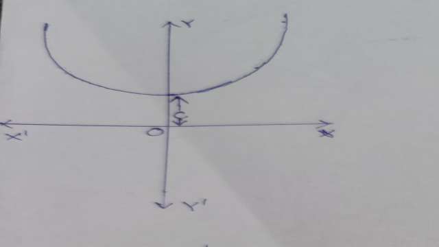
Example-2. सिद्ध कीजिए कि कैटिनरी y=c\cosh { \left( \frac { x }{ c } \right) } के शीर्ष (0,c) से किसी अन्य बिन्दु तक के चाप की लम्बाई s=c\sinh { \left( \frac { x }{ c } \right) } है।
(Prove that length of the arc of the catenary y=c\cosh { \left( \frac { x }{ c } \right) } from the vertex (0,c) to any other point is s=c\sinh { \left( \frac { x }{ c } \right) } .)

Solution– दिए हुए वक्र का समीकरण-

y=c\cosh { \left( \frac { x }{ c } \right) } \\ \frac { dy }{ dx } =\sinh { \left( \frac { x }{ c } \right) }
समाकलन की सीमाएं x=0 से x=x है।
अतः चाप की लम्बाई s={ \int }_{ 0 }^{ x }\sqrt { 1+{ \left( \frac { dy }{ dx } \right) }^{ 2 } } dx\\ ={ \int }_{ 0 }^{ x }\sqrt { 1+\sinh ^{ 2 }{ \left( \frac { x }{ c } \right) } } dx\\ ={ \int }_{ 0 }^{ x }\sqrt { \cosh ^{ 2 }{ \left( \frac { x }{ c } \right) } } dx\\ ={ \int }_{ 0 }^{ x }\cosh { \left( \frac { x }{ c } \right) } dx\\ ={ \left[ \sinh { \left( \frac { x }{ c } \right) } \right] }_{ 0 }^{ x }\\ =\sinh { \left( \frac { x }{ c } \right) }

उपर्युक्त उदाहरण के द्वारा समतल वक्रों की लम्बाईयां (Lengths of Plane Curves) को समझ सकते हैं।
Example-3. वक्र { x }^{ 2 }\left( { a }^{ 2 }-{ x }^{ 2 } \right) =8{ a }^{ 2 }{ y }^{ 2 } की सम्पूर्ण लम्बाई ज्ञात कीजिए।
(Find the whole length of the curve { x }^{ 2 }\left( { a }^{ 2 }-{ x }^{ 2 } \right) =8{ a }^{ 2 }{ y }^{ 2 }.)
Solution- वक्र का समीकरण-

{ x }^{ 2 }\left( { a }^{ 2 }-{ x }^{ 2 } \right) =8{ a }^{ 2 }{ y }^{ 2 }\\ \Rightarrow 8{ a }^{ 2 }{ y }^{ 2 }={ x }^{ 2 }\left( { a }^{ 2 }-{ x }^{ 2 } \right) \\ \Rightarrow { y }^{ 2 }=\frac { { x }^{ 2 }\left( { a }^{ 2 }-{ x }^{ 2 } \right) }{ 8{ a }^{ 2 } } \\ \Rightarrow y=\frac { 1 }{ 2\sqrt { 2 } a } x\sqrt { { a }^{ 2 }-{ x }^{ 2 } }

x के सापेक्ष अवकलन करने पर –

\frac { dy }{ dx } =\frac { 1 }{ 2\sqrt { 2 } a } \left[ \sqrt { { a }^{ 2 }-{ x }^{ 2 } } +x.\frac { 1 }{ 2\sqrt { { a }^{ 2 }-{ x }^{ 2 } } } \left( -2x \right) \right] \\ \frac { dy }{ dx } =\frac { 1 }{ 2\sqrt { 2 } a } \left[ \sqrt { { a }^{ 2 }-{ x }^{ 2 } } -\frac { { x }^{ 2 } }{ \sqrt { { a }^{ 2 }-{ x }^{ 2 } } } \right] \\ \frac { dy }{ dx } =\frac { 1 }{ 2\sqrt { 2 } a } \left[ \frac { { a }^{ 2 }-{ x }^{ 2 }-{ x }^{ 2 } }{ \sqrt { { a }^{ 2 }-{ x }^{ 2 } } } \right] \\ \frac { dy }{ dx } =\frac { 1 }{ 2\sqrt { 2 } a } \left[ \frac { { a }^{ 2 }-2{ x }^{ 2 } }{ \sqrt { { a }^{ 2 }-{ x }^{ 2 } } } \right]
समाकलन की सीमाएं x=0 से x=a हैं।
अतः सम्पूर्ण चाप की लम्बाई s=4{ \int }_{ 0 }^{ a }\sqrt { 1+{ \left( \frac { dy }{ dx } \right) }^{ 2 } } dx\\ =4{ \int }_{ 0 }^{ a }\sqrt { 1+\frac { { \left( { a }^{ 2 }-2{ x }^{ 2 } \right) }^{ 2 } }{ 8{ a }^{ 2 }\left( { a }^{ 2 }-{ x }^{ 2 } \right) } } dx\\ =4{ \int }_{ 0 }^{ a }\sqrt { \frac { 8{ a }^{ 4 }-8{ a }^{ 2 }{ x }^{ 2 }+{ a }^{ 4 }-4{ a }^{ 2 }{ x }^{ 2 }+4{ x }^{ 4 } }{ 8{ a }^{ 2 }\left( { a }^{ 2 }-{ x }^{ 2 } \right) } } dx\\ =4{ \int }_{ 0 }^{ a }\sqrt { \frac { 9{ a }^{ 4 }-12{ a }^{ 2 }{ x }^{ 2 }+4{ x }^{ 4 } }{ 8{ a }^{ 2 }\left( { a }^{ 2 }-{ x }^{ 2 } \right) } } dx\\ =\frac { 4 }{ 2\sqrt { 2 } a } { \int }_{ 0 }^{ a }\sqrt { \frac { { \left( 3{ a }^{ 2 }-2{ x }^{ 2 } \right) }^{ 2 } }{ \left( { a }^{ 2 }-{ x }^{ 2 } \right) } } dx\\ =\frac { \sqrt { 2 } }{ a } { \int }_{ 0 }^{ a }\frac { { \left( 3{ a }^{ 2 }-2{ x }^{ 2 } \right) } }{ \sqrt { { a }^{ 2 }-{ x }^{ 2 } } } dx\\ =\frac { \sqrt { 2 } }{ a } { \int }_{ 0 }^{ a }\frac { { \left( { a }^{ 2 }+2{ a }^{ 2 }-2{ x }^{ 2 } \right) } }{ \sqrt { { a }^{ 2 }-{ x }^{ 2 } } } dx\\ =\frac { \sqrt { 2 } }{ a } { \int }_{ 0 }^{ a }\left[ \frac { { a }^{ 2 } }{ \sqrt { { a }^{ 2 }-{ x }^{ 2 } } } -\frac { 2\left( { a }^{ 2 }-{ x }^{ 2 } \right) }{ \sqrt { { a }^{ 2 }-{ x }^{ 2 } } } \right] dx\\ =\frac { \sqrt { 2 } { a }^{ 2 } }{ a } { \int }_{ 0 }^{ a }\frac { 1 }{ \sqrt { { a }^{ 2 }-{ x }^{ 2 } } } dx+\frac { 2\sqrt { 2 } }{ a } { \int }_{ 0 }^{ a }\sqrt { { a }^{ 2 }-{ x }^{ 2 } } dx\\ =\sqrt { 2 } a{ \left[ \sin ^{ -1 }{ \frac { x }{ a } } \right] }_{ 0 }^{ a }+\frac { 2\sqrt { 2 } }{ a } { \left[ \frac { x }{ 2 } \sqrt { { a }^{ 2 }-{ x }^{ 2 } } +\frac { { a }^{ 2 } }{ 2 } \sin ^{ -1 }{ \frac { x }{ a } } \right] }_{ 0 }^{ a }\\ =\sqrt { 2 } a\left( \sin ^{ -1 }{ 1 } \right) +\frac { 2\sqrt { 2 } }{ a } \left[ \frac { { a }^{ 2 } }{ 2 } \sin ^{ -1 }{ 1 } \right] \\ =\sqrt { 2 } a\left( \frac { \pi }{ 2 } \right) +\frac { 2\sqrt { 2 } }{ a } .\frac { \pi }{ 2 } \\ =\frac { \pi a }{ \sqrt { 2 } } +\frac { \pi a }{ \sqrt { 2 } } \\ =\frac { 2\pi a }{ \sqrt { 2 } } \\ S=\sqrt { 2 } \pi a

उपर्युक्त उदाहरण के द्वारा समतल वक्रों की लम्बाईयां (Lengths of Plane Curves) को समझ सकते हैं।
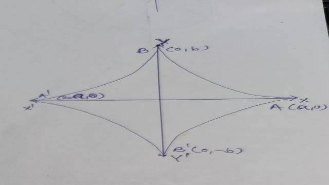
Example-4. वक्र { \left( \frac { x }{ a } \right) }^{ \frac { 2 }{ 3 } }+{ \left( \frac { y }{ b } \right) }^{ \frac { 2 }{ 3 } }=1 की सम्पूर्ण लम्बाई ज्ञात कीजिए:
(Find the whole length of the curve { \left( \frac { x }{ a } \right) }^{ \frac { 2 }{ 3 } }+{ \left( \frac { y }{ b } \right) }^{ \frac { 2 }{ 3 } }=1.)

Solution– वक्र का समीकरण-

{ \left( \frac { x }{ a } \right) }^{ \frac { 2 }{ 3 } }+{ \left( \frac { y }{ b } \right) }^{ \frac { 2 }{ 3 } }=1
वक्र का प्राचलिक समीकरण-

x=a\cos ^{ 3 }{ \theta } ,y=\sin ^{ 3 }{ \theta } \\ \frac { dx }{ d\theta } =-3a\cos ^{ 2 }{ \theta } \sin { \theta } ,\frac { dy }{ d\theta } =3b\sin ^{ 2 }{ \theta } \cos { \theta }
प्रथम चतुर्थांश में समाकलन की सीमाएं \theta =0 से \theta =\frac { \pi }{ 2 } हैं।
अतः सम्पूर्ण चाप की लम्बाई s=4{ \int }_{ 0 }^{ \frac { \pi }{ 2 } }\sqrt { { \left( \frac { dx }{ d\theta } \right) }^{ 2 }+{ \left( \frac { dy }{ d\theta } \right) }^{ 2 } } d\theta \\ =4{ \int }_{ 0 }^{ \frac { \pi }{ 2 } }\sqrt { { \left( -3a\cos ^{ 2 }{ \theta } \sin { \theta } \right) }^{ 2 }+{ \left( 3b\sin ^{ 2 }{ \theta } \cos { \theta } \right) }^{ 2 } } d\theta \\ =4{ \int }_{ 0 }^{ \frac { \pi }{ 2 } }\sqrt { 9{ a }^{ 2 }\cos ^{ 4 }{ \theta } \sin ^{ 2 }{ \theta } +9{ b }^{ 2 }\sin ^{ 4 }{ \theta } \cos ^{ 2 }{ \theta } } d\theta \\ =4{ \int }_{ 0 }^{ \frac { \pi }{ 2 } }\sqrt { 9\cos ^{ 2 }{ \theta } \sin ^{ 2 }{ \theta } \left( { a }^{ 2 }\cos ^{ 2 }{ \theta } +{ b }^{ 2 }\sin ^{ 2 }{ \theta } \right) } d\theta \\ =4{ \int }_{ 0 }^{ \frac { \pi }{ 2 } }3\sin { \theta } \cos { \theta } \sqrt { \left( { a }^{ 2 }\cos ^{ 2 }{ \theta } +{ b }^{ 2 }\sin ^{ 2 }{ \theta } \right) } d\theta \\ put\quad \left( { a }^{ 2 }\cos ^{ 2 }{ \theta } +{ b }^{ 2 }\sin ^{ 2 }{ \theta } \right) ={ t }^{ 2 }\\ \Rightarrow \left( -2{ a }^{ 2 }\cos { \theta } \sin { \theta } +2{ b }^{ 2 }\sin { \theta } \cos { \theta } \right) d\theta =2tdt\\ \Rightarrow 2\left( { b }^{ 2 }-{ a }^{ 2 } \right) \sin { \theta } \cos { \theta } d\theta =2tdt\\ \Rightarrow \left( { b }^{ 2 }-{ a }^{ 2 } \right) \sin { \theta } \cos { \theta } d\theta =tdt\\ \Rightarrow \sin { \theta } \cos { \theta } d\theta =\frac { tdt }{ \left( { b }^{ 2 }-{ a }^{ 2 } \right) }
जब \theta =0 तो t=a
जब \theta =\frac { \pi }{ 2 }  तो t=b

s=12{ \int }_{ a }^{ b }\sqrt { { t }^{ 2 } } .\frac { tdt }{ \left( { b }^{ 2 }-{ a }^{ 2 } \right) } \\ s=\frac { 12 }{ \left( { b }^{ 2 }-{ a }^{ 2 } \right) } { \int }_{ a }^{ b }{ t }^{ 2 }dt\\ s=\frac { 12 }{ \left( { b }^{ 2 }-{ a }^{ 2 } \right) } { \left[ \frac { { t }^{ 3 } }{ 3 } \right] }_{ a }^{ b }\\ s=\frac { 12 }{ \left( { b }^{ 2 }-{ a }^{ 2 } \right) } .\frac { 1 }{ 3 } \left[ { b }^{ 3 }-{ a }^{ 3 } \right] \\ s=\frac { 4 }{ \left( b-a \right) \left( a+b \right) } \left( b-a \right) \left( { b }^{ 2 }+{ a }^{ 2 }+ab \right) \\ s=\frac { 4\left( { a }^{ 2 }+{ b }^{ 2 }+ab \right) }{ \left( a+b \right) }

उपर्युक्त उदाहरण के द्वारा समतल वक्रों की लम्बाईयां (Lengths of Plane Curves) को समझ सकते हैं।
Example-5.सिद्ध कीजिए कि वक्र x={ t }^{ 2 },y=t-\frac { { t }^{ 3 } }{ 3 } के लूप का परिमाप 4\sqrt { 3 }  है।
(Prove that the perimeter of the loop of the curve x={ t }^{ 2 },y=t-\frac { { t }^{ 3 } }{ 3 } is 4\sqrt { 3 } .)
Solution– वक्र का समीकरण-

x={ t }^{ 2 },y=t-\frac { { t }^{ 3 } }{ 3 } \\ \frac { dx }{ dt } =2t,\frac { dy }{ dt } =1-{ t }^{ 2 }
समाकलन की सीमाएं ज्ञात करने के लिए y=0 रखने पर-

t-\frac { { t }^{ 3 } }{ 3 } =0\\ \Rightarrow t\left( 1-\frac { { t }^{ 2 } }{ 3 } \right) =0\\ \Rightarrow t=0,t=\sqrt { 3 }
अतः लूप का परिमाप s=2{ \int }_{ 0 }^{ \sqrt { 3 } }\sqrt { { \left( \frac { dx }{ dt } \right) }^{ 2 }+{ \left( \frac { dy }{ dt } \right) }^{ 2 } } dt\\ s=2{ \int }_{ 0 }^{ \sqrt { 3 } }\sqrt { { \left( 2t \right) }^{ 2 }+{ \left( 1-{ t }^{ 2 } \right) }^{ 2 } } dt\\ s=2{ \int }_{ 0 }^{ \sqrt { 3 } }\sqrt { 4{ t }^{ 2 }+1-2{ t }^{ 2 }+{ t }^{ 4 } } dt\\ s=2{ \int }_{ 0 }^{ \sqrt { 3 } }\sqrt { 1+2{ t }^{ 2 }+{ t }^{ 4 } } dt\\ s=2{ \int }_{ 0 }^{ \sqrt { 3 } }\sqrt { { \left( 1+{ t }^{ 2 } \right) }^{ 2 } } dt\\ s=2{ \int }_{ 0 }^{ \sqrt { 3 } }\left( 1+{ t }^{ 2 } \right) dt\\ s=2{ \left[ t+\frac { { t }^{ 3 } }{ 3 } \right] }_{ 0 }^{ \sqrt { 3 } }\\ s=2\left[ \sqrt { 3 } +\sqrt { 3 } \right] \\ s=4\sqrt { 3 }

उपर्युक्त उदाहरण के द्वारा समतल वक्रों की लम्बाईयां (Lengths of Plane Curves) को समझ सकते हैं।
Example-6.वक्र x={ e }^{ \theta }\left( \sin { \frac { \theta }{ 2 } } +2\cos { \frac { \theta }{ 2 } } \right) ,y={ e }^{ \theta }\left( \cos { \frac { \theta }{ 2 } } -2\sin { \frac { \theta }{ 2 } } \right) की \theta =0 से \theta =\pi  तक की लम्बाई ज्ञात कीजिए।
(Find the length of the curve x={ e }^{ \theta }\left( \sin { \frac { \theta }{ 2 } } +2\cos { \frac { \theta }{ 2 } } \right) ,y={ e }^{ \theta }\left( \cos { \frac { \theta }{ 2 } } -2\sin { \frac { \theta }{ 2 } } \right) from \theta =0 to \theta =\pi .)
Solution- वक्र का प्राचलिक समीकरण-

x={ e }^{ \theta }\left( \sin { \frac { \theta }{ 2 } } +2\cos { \frac { \theta }{ 2 } } \right) ,y={ e }^{ \theta }\left( \cos { \frac { \theta }{ 2 } } -2\sin { \frac { \theta }{ 2 } } \right) \\ \frac { dx }{ d\theta } ={ e }^{ \theta }\left( \sin { \frac { \theta }{ 2 } } +2\cos { \frac { \theta }{ 2 } } \right) +{ e }^{ \theta }\left( \frac { 1 }{ 2 } \cos { \frac { \theta }{ 2 } } -\sin { \frac { \theta }{ 2 } } \right) \\ \Rightarrow \frac { dx }{ d\theta } =\frac { 5 }{ 2 } { e }^{ \theta }\cos { \frac { \theta }{ 2 } } \\ \frac { dy }{ d\theta } ={ e }^{ \theta }\left( \cos { \frac { \theta }{ 2 } } -2\sin { \frac { \theta }{ 2 } } \right) +{ e }^{ \theta }\left( -\frac { 1 }{ 2 } \sin { \frac { \theta }{ 2 } } -\cos { \frac { \theta }{ 2 } } \right) \\ \Rightarrow \frac { dy }{ d\theta } =-\frac { 5 }{ 2 } { e }^{ \theta }\left( \sin { \frac { \theta }{ 2 } } \right)
समाकलन की सीमाएं \theta =0 से \theta =\pi  हैं।
अतः चाप की लम्बाई s={ \int }_{ 0 }^{ \pi }\sqrt { { \left( \frac { dx }{ d\theta } \right) }^{ 2 }+{ \left( \frac { dy }{ d\theta } \right) }^{ 2 } } d\theta \\ s={ \int }_{ 0 }^{ \pi }\sqrt { { \left( \frac { 5 }{ 2 } { e }^{ \theta }\cos { \frac { \theta }{ 2 } } \right) }^{ 2 }+{ \left( \frac { 5 }{ 2 } { e }^{ \theta }\sin { \frac { \theta }{ 2 } } \right) }^{ 2 } } d\theta \\ \Rightarrow s={ \int }_{ 0 }^{ \pi }\sqrt { \frac { 25 }{ 4 } { e }^{ 2\theta }\left( \cos ^{ 2 }{ \frac { \theta }{ 2 } } +\sin ^{ 2 }{ \frac { \theta }{ 2 } } \right) } d\theta \\ \Rightarrow s={ \int }_{ 0 }^{ \pi }\frac { 5 }{ 2 } { e }^{ \theta }\sqrt { \left( \cos ^{ 2 }{ \frac { \theta }{ 2 } } +\sin ^{ 2 }{ \frac { \theta }{ 2 } } \right) } d\theta \\ \Rightarrow s=\frac { 5 }{ 2 } { \int }_{ 0 }^{ \pi }{ e }^{ \theta }d\theta \\ \Rightarrow s=\frac { 5 }{ 2 } { \left[ { e }^{ \theta } \right] }_{ 0 }^{ \pi }\\ \Rightarrow s=\frac { 5 }{ 2 } \left( { e }^{ \pi }-1 \right)

उपर्युक्त उदाहरण के द्वारा समतल वक्रों की लम्बाईयां (Lengths of Plane Curves) को समझ सकते हैं।
Example-7. सिद्ध कीजिए कि वक्र के चाप की लम्बाई
Prove that the length of the arc of the curve

x=a\left( 3\sin { \theta } -\sin ^{ 3 }{ \theta } \right) ,y=a\cos ^{ 3 }{ \theta }
जो कि (0,a) से किसी बिन्दु (x,y) तक नापा गया है,\frac { 3 }{ 2 } \left( \theta +\sin { \theta } \cos { \theta } \right) है।
(Which is measured from (0,a) to any point (x,y) is \frac { 3 }{ 2 } \left( \theta +\sin { \theta } \cos { \theta } \right) .)
Solution– वक्र का प्राचलिक समीकरण-

x=a\left( 3\sin { \theta } -\sin ^{ 3 }{ \theta } \right) ,y=a\cos ^{ 3 }{ \theta } \qquad \\ \frac { dx }{ d\theta } =a\left( 3\cos { \theta } -3\sin ^{ 3 }{ \theta } \cos { \theta } \right) ,\frac { dy }{ d\theta } =-3a\cos ^{ 2 }{ \theta } \sin { \theta }
समाकलन की सीमाएं \theta =0 से \theta हैं।
चाप की लम्बाई s={ \int }_{ 0 }^{ \theta }\sqrt { { \left( \frac { dx }{ d\theta } \right) }^{ 2 }+{ \left( \frac { dy }{ d\theta } \right) }^{ 2 } } d\theta \\ \Rightarrow s={ \int }_{ 0 }^{ \theta }\sqrt { { \left\{ a\left( 3\cos { \theta } -3\sin ^{ 3 }{ \theta } \cos { \theta } \right) \right\} }^{ 2 }+{ \left\{ -3a\cos ^{ 2 }{ \theta } \sin { \theta } \right\} }^{ 2 } } d\theta \\ \Rightarrow s={ \int }_{ 0 }^{ \theta }\sqrt { { a }^{ 2 }.9\cos ^{ 2 }{ \theta } { \left( 1-\sin ^{ 2 }{ \theta } \right) }^{ 2 }+9a^{ 2 }\cos ^{ 4 }{ \theta } \sin ^{ 2 }{ \theta } } d\theta \\ \Rightarrow s={ 3a\int }_{ 0 }^{ \theta }\sqrt { \cos ^{ 2 }{ \theta } { \left( \cos ^{ 2 }{ \theta } \right) }^{ 2 }+\cos ^{ 4 }{ \theta } \sin ^{ 2 }{ \theta } } d\theta \\ \Rightarrow s={ 3a\int }_{ 0 }^{ \theta }\sqrt { \cos ^{ 2 }{ \theta } .\cos ^{ 4 }{ \theta } +\cos ^{ 4 }{ \theta } \sin ^{ 2 }{ \theta } } d\theta \\ \Rightarrow s={ 3a\int }_{ 0 }^{ \theta }\sqrt { \cos ^{ 4 }{ \theta } \left( \cos ^{ 2 }{ \theta } +\sin ^{ 2 }{ \theta } \right) } d\theta \\ \Rightarrow s={ 3a\int }_{ 0 }^{ \theta }\cos ^{ 2 }{ \theta } d\theta \\ \Rightarrow s={ 3a\int }_{ 0 }^{ \theta }\left( \frac { 1+\cos { 2\theta } }{ 2 } \right) d\theta \\ \Rightarrow s=\frac { 3a }{ 2 } { \int }_{ 0 }^{ \theta }\left( 1+\cos { 2\theta } \right) d\theta \\ \Rightarrow s=\frac { 3a }{ 2 } { \left[ \theta +\frac { \sin { 2\theta } }{ 2 } \right] }_{ 0 }^{ \theta }\\ \Rightarrow s=\frac { 3a }{ 2 } { \left[ \theta +\frac { 2\sin { \theta } \cos { \theta } }{ 2 } \right] }\\ \Rightarrow s=\frac { 3a }{ 2 } { \left[ \theta +\sin { \theta } \cos { \theta } \right] }

उपर्युक्त उदाहरण के द्वारा समतल वक्रों की लम्बाईयां (Lengths of Plane Curves) को समझ सकते हैं।
Example-8. परवलय \frac { l }{ r } =1+\cos { \theta } के नाभिलम्ब द्वारा काटे गए चाप की लम्बाई ज्ञात कीजिए।
(Find the length of the arc of parabola \frac { l }{ r } =1+\cos { \theta } intercepted by the latus rectum.)

Solution– O ध्रुव है तथा LOL’ परवलय का नाभिलम्ब है।
परवलय का समीकरण-

\frac { l }{ r } =1+\cos { \theta } \\ \Rightarrow r=\frac { l }{ 1+\cos { \theta } } \\ \Rightarrow r=\frac { l }{ 2\cos ^{ 2 }{ \frac { \theta }{ 2 } } } \\ \Rightarrow r=\frac { l }{ 2 } \sec ^{ 2 }{ \frac { \theta }{ 2 } } \\ \Rightarrow \frac { dr }{ d\theta } =\frac { l }{ 2 } .2\sec { \frac { \theta }{ 2 } } \sec { \frac { \theta }{ 2 } } \tan { \frac { \theta }{ 2 } } \frac { 1 }{ 2 } \\ \Rightarrow \frac { dr }{ d\theta } =\frac { l }{ 2 } .\sec ^{ 2 }{ \frac { \theta }{ 2 } } \tan { \frac { \theta }{ 2 } }
अतः नाभिलम्ब द्वारा काटे गए चाप की लम्बाई s=\int _{ 0 }^{ \frac { \pi }{ 2 } }{ 2\sqrt { { r }^{ 2 }+{ (\frac { dr }{ d\theta } ) }^{ 2 } } d\theta } \\ =2\int _{ 0 }^{ \frac { \pi }{ 2 } }{ \sqrt { \frac { { l }^{ 2 } }{ { (1+\cos { \theta } ) }^{ 2 } } +\frac { { l }^{ 2 } }{ 4 } \sec ^{ 4 }{ \frac { \theta }{ 2 } } \tan ^{ 2 }{ \frac { \theta }{ 2 } } } d\theta } \\ =2\int _{ 0 }^{ \frac { \pi }{ 2 } }{ \sqrt { \frac { { l }^{ 2 } }{ 4\cos ^{ 4 }{ \frac { \theta }{ 2 } } } +\frac { { l }^{ 2 } }{ 4 } \sec ^{ 4 }{ \frac { \theta }{ 2 } } \tan ^{ 2 }{ \frac { \theta }{ 2 } } } d\theta } \\ =2\int _{ 0 }^{ \frac { \pi }{ 2 } }{ \frac { l }{ 2 } \sqrt { (\sec ^{ 4 }{ \frac { \theta }{ 2 } } +\sec ^{ 4 }{ \frac { \theta }{ 2 } } \tan ^{ 2 }{ \frac { \theta }{ 2 } } ) } d\theta } \\ =l\int _{ 0 }^{ \frac { \pi }{ 2 } }{ \sqrt { \sec ^{ 4 }{ \frac { \theta }{ 2 } } (1+\tan ^{ 2 }{ \frac { \theta }{ 2 } } ) } d\theta } \\ =l\int _{ 0 }^{ \frac { \pi }{ 2 } }{ \sqrt { \sec ^{ 4 }{ \frac { \theta }{ 2 } } \sec ^{ 2 }{ \frac { \theta }{ 2 } } } d\theta } \\ =l\int _{ 0 }^{ \frac { \pi }{ 2 } }{ \sqrt { \sec ^{ 6 }{ \frac { \theta }{ 2 } } } d\theta } \\ =l\int _{ 0 }^{ \frac { \pi }{ 2 } }{ \sec ^{ 3 }{ \frac { \theta }{ 2 } } d\theta } \\ \Rightarrow s=l\int _{ 0 }^{ \frac { \pi }{ 2 } }{ \sec ^{ 3 }{ \frac { \theta }{ 2 } } d\theta } .....(1)\\ माना\quad I=\int { \sec ^{ 3 }{ \frac { \theta }{ 2 } } d\theta } \\ I=\int { \sec { \frac { \theta }{ 2 } } \sec ^{ 2 }{ \frac { \theta }{ 2 } } d\theta } \\ I=\sec { \frac { \theta }{ 2 } } \int { \sec ^{ 2 }{ \frac { \theta }{ 2 } } d\theta } -\int { [\frac { d }{ d\theta } \sec { \frac { \theta }{ 2 } } \int { \sec ^{ 2 }{ \frac { \theta }{ 2 } } } ]d\theta } \\ I=2\sec { \frac { \theta }{ 2 } } \tan { \frac { \theta }{ 2 } } -\int { \sec { \frac { \theta }{ 2 } } \tan { \frac { \theta }{ 2 } } \tan { \frac { \theta }{ 2 } } d\theta } \\ I=2\sec { \frac { \theta }{ 2 } } \tan { \frac { \theta }{ 2 } } -\int { \sec { \frac { \theta }{ 2 } } \tan ^{ 2 }{ \frac { \theta }{ 2 } } d\theta } \\ I=2\sec { \frac { \theta }{ 2 } } \tan { \frac { \theta }{ 2 } } -\int { \sec { \frac { \theta }{ 2 } } (\sec ^{ 2 }{ \frac { \theta }{ 2 } } -1)d\theta } \\ I=2\sec { \frac { \theta }{ 2 } } \tan { \frac { \theta }{ 2 } } -\int { \sec ^{ 3 }{ \frac { \theta }{ 2 } } } d\theta +\int { \sec { \frac { \theta }{ 2 } } d\theta } \\ I=2\sec { \frac { \theta }{ 2 } } \tan { \frac { \theta }{ 2 } } -I+2\log { (\sec { \frac { \theta }{ 2 } } +\tan { \frac { \theta }{ 2 } } ) } \\ \Rightarrow 2I=2\sec { \frac { \theta }{ 2 } } \tan { \frac { \theta }{ 2 } } +2\log { (\sec { \frac { \theta }{ 2 } } +\tan { \frac { \theta }{ 2 } } ) } \\ \Rightarrow I=\sec { \frac { \theta }{ 2 } } \tan { \frac { \theta }{ 2 } } +\log { (\sec { \frac { \theta }{ 2 } } +\tan { \frac { \theta }{ 2 } } ) }
समीकरण (1) में मान रखने पर-

s=l{ [\sec { \frac { \theta }{ 2 } } \tan { \frac { \theta }{ 2 } } +\log { (\sec { \frac { \theta }{ 2 } } +\tan { \frac { \theta }{ 2 } } ) } ] }_{ 0 }^{ \frac { \pi }{ 2 } }\\ \Rightarrow s=l[\sec { \frac { \pi }{ 4 } } \tan { \frac { \pi }{ 4 } } +\log { (\sec { \frac { \pi }{ 4 } } +\tan { \frac { \pi }{ 4 } } ) } ]\\ \Rightarrow s=l[\sqrt { 2 } +\log { (\sqrt { 2 } +1) } ]

उपर्युक्त उदाहरण के द्वारा समतल वक्रों की लम्बाईयां (Lengths of Plane Curves) को समझ सकते हैं।
Example-9. प्रदर्शित कीजिए कि लिमकेन r=a+b\cos { \theta } (a>b) की सम्पूर्ण लम्बाई उस दीर्घवृत्त की परिमाप के बराबर है जिसकी अर्द्ध-अक्षें लिमकेन के अधिकतम एवं लघुत्तम ध्रुवान्तर है।
(Show that the whole length of the limacon r=a+b\cos { \theta } (a>b) is equal to the perimeter of an ellipse whose semi-axes are maximum and minimum radii vector of limacon.)

Solution- लिमेकन की समीकरण-

r=a+b\cos { \theta } \\ \frac { dr }{ d\theta } =-b\sin { \theta }
लिमेकन का परिमाप { S }_{ 1 }=2\int _{ 0 }^{ \pi }{ \sqrt { { r }^{ 2 }+{ (\frac { dr }{ d\theta } ) }^{ 2 }d\theta } } \\ =2\int _{ 0 }^{ \pi }{ \sqrt { { (a+b\cos { \theta } ) }^{ 2 }+{ b }^{ 2 }\sin ^{ 2 }{ \theta } d\theta } } \\ =2\int _{ 0 }^{ \pi }{ \sqrt { { a }^{ 2 }+2ab\cos { \theta } +{ b }^{ 2 }\cos ^{ 2 }{ \theta } +{ b }^{ 2 }\sin ^{ 2 }{ \theta } } } d\theta \\ =2\int _{ 0 }^{ \pi }{ \sqrt { { a }^{ 2 }+2ab\cos { \theta } +{ b }^{ 2 } } } d\theta \\ =2a\int _{ 0 }^{ \pi }{ \sqrt { 1+2\frac { b }{ a } \cos { \theta } +\frac { { b }^{ 2 } }{ { a }^{ 2 } } } } d\theta \\ =2a\int _{ 0 }^{ \pi }{ { [1+\frac { 2b }{ a } \cos { \theta } +\frac { { b }^{ 2 } }{ { a }^{ 2 } } ] }^{ \frac { 1 }{ 2 } } } d\theta \\ =2a\int _{ 0 }^{ \pi }{ { [1+ } } \frac { b }{ a } \cos { \theta } +\frac { 1 }{ 2 } \frac { { b }^{ 2 } }{ { a }^{ 2 } } +\frac { \frac { 1 }{ 2 } (\frac { 1 }{ 2 } -1) }{ 2! } { (\frac { 2b }{ a } \cos { \theta } +\frac { { b }^{ 2 } }{ { a }^{ 2 } } ) }^{ 2 }+.....]d\theta \\ =2a\int _{ 0 }^{ \pi }{ { [1+ } } \frac { b }{ a } \cos { \theta } +\frac { { b }^{ 2 } }{ 2{ a }^{ 2 } } -\frac { 1 }{ 8 } .\frac { { 4b }^{ 2 } }{ { a }^{ 2 } } \cos ^{ 2 }{ \theta } -\frac { 1 }{ 8 } \frac { { b }^{ 4 } }{ { a }^{ 4 } } -\frac { 1 }{ 8 } \frac { { 4b }^{ 3 } }{ { a }^{ 3 } } \cos { \theta } +....]d\theta

[उच्चतम घातों को छोड़ने  पर  ]

{ S }_{ 1 }=2a\int _{ 0 }^{ \pi }{ { [1+\frac { b }{ a } \cos { \theta } +\frac { { b }^{ 2 } }{ 2{ a }^{ 2 } } -\frac { 1 }{ 2 } .\frac { { b }^{ 2 } }{ { a }^{ 2 } } \cos ^{ 2 }{ \theta } ] } } d\theta \\ =2a\int _{ 0 }^{ \pi }{ { [1+\frac { b }{ a } \cos { \theta } +\frac { { b }^{ 2 } }{ 2{ a }^{ 2 } } (1-\cos ^{ 2 }{ \theta } )] } } d\theta \\ =2a\int _{ 0 }^{ \pi }{ { [1+\frac { b }{ a } \cos { \theta } +\frac { { b }^{ 2 } }{ 2{ a }^{ 2 } } \sin ^{ 2 }{ \theta } ] } } d\theta \\ =2a\int _{ 0 }^{ \pi }{ { [1+\frac { b }{ a } \cos { \theta } +\frac { { b }^{ 2 } }{ 2{ a }^{ 2 } } (\frac { 1-\cos { 2\theta } }{ 2 } )] } } d\theta \\ \Rightarrow { S }_{ 1 }=2a\int _{ 0 }^{ \pi }{ { [1+\frac { { b }^{ 2 } }{ 4{ a }^{ 2 } } +\frac { b }{ a } \cos { \theta } -\frac { { b }^{ 2 } }{ 4{ a }^{ 2 } } \cos { 2\theta } ] } } d\theta \\ \Rightarrow { S }_{ 1 }=2a{ [\theta +\frac { { b }^{ 2 } }{ 4{ a }^{ 2 } } \theta +\frac { b }{ a } \sin { \theta } -\frac { { b }^{ 2 } }{ 8{ a }^{ 2 } } \sin { 2\theta } ] }_{ 0 }^{ \pi }\\ \Rightarrow { S }_{ 1 }=2a{ [\pi +\frac { { b }^{ 2 } }{ 4{ a }^{ 2 } } \pi ] }\\ \Rightarrow { S }_{ 1 }=2\pi a{ [1+\frac { { b }^{ 2 } }{ 4{ a }^{ 2 } } ] }
दीर्घवृत्त का प्राचलिक समीकरण-

x=(a+b)\cos { \theta } ,y=(a-b)\sin { \theta } \\ \frac { dx }{ d\theta } =-(a+b)\sin { \theta } ,\frac { dy }{ d\theta } =(a-b)\cos { \theta }
दीर्घवृत्त का परिमाप

{ S }_{ 2 }=4\int _{ 0 }^{ \frac { \pi }{ 2 } }{ \sqrt { { (\frac { dx }{ d\theta } ) }^{ 2 }+{ (\frac { dy }{ d\theta } ) }^{ 2 }d\theta } } \\ { S }_{ 2 }=4\int _{ 0 }^{ \frac { \pi }{ 2 } }{ \sqrt { { (a+b) }^{ 2 }\sin ^{ 2 }{ \theta } +{ (a-b) }^{ 2 }\cos ^{ 2 }{ \theta } } } d\theta \\ { S }_{ 2 }=4\int _{ 0 }^{ \frac { \pi }{ 2 } }{ \sqrt { \begin{matrix} { a }^{ 2 }\sin ^{ 2 }{ \theta } +{ b }^{ 2 }\sin ^{ 2 }{ \theta } +2ab\sin ^{ 2 }{ \theta } \\ +{ a }^{ 2 }\cos ^{ 2 }{ \theta } +{ b }^{ 2 }\cos ^{ 2 }{ \theta } +2ab\cos ^{ 2 }{ \theta } \end{matrix} } } d\theta \\ { S }_{ 2 }=4\int _{ 0 }^{ \frac { \pi }{ 2 } }{ \sqrt { { a }^{ 2 }+{ b }^{ 2 }+2ab\cos { 2\theta } } } d\theta \\ =4\int _{ 0 }^{ \frac { \pi }{ 2 } }{ a{ [1+\frac { { b }^{ 2 } }{ { a }^{ 2 } } +\frac { 2b }{ a } \cos { 2\theta } ] }^{ \frac { 1 }{ 2 } } } d\theta \\ =4a\int _{ 0 }^{ \pi }{ { [1+ } } \frac { { b }^{ 2 } }{ { 2a }^{ 2 } } -\frac { b }{ a } \cos { 2\theta } +\frac { \frac { 1 }{ 2 } (\frac { 1 }{ 2 } -1) }{ 2! } { (\frac { { b }^{ 2 } }{ { a }^{ 2 } } -\frac { 2b }{ a } \cos { \theta } ) }^{ 2 }+.....]d\theta \\ =4a\int _{ 0 }^{ \pi }{ { [1+ } } \frac { { b }^{ 2 } }{ { 2a }^{ 2 } } -\frac { b }{ a } \cos { 2\theta } -\frac { 1 }{ 8 } (\frac { { b }^{ 4 } }{ { a }^{ 4 } } +\frac { { 4b }^{ 2 } }{ { a }^{ 2 } } \cos ^{ 2 }{ 2\theta } -\frac { { 4b }^{ 3 } }{ { a }^{ 3 } } \cos { 2\theta } +....]d\theta

[उच्चतम घातों को छोड़ने  पर  ]

{ S }_{ 2 }=4a\int _{ 0 }^{ \pi }{ { [1+\frac { { b }^{ 2 } }{ { 2a }^{ 2 } } -\frac { b }{ a } \cos { 2\theta } -\frac { { b }^{ 2 } }{ { 2a }^{ 2 } } \cos ^{ 2 }{ 2\theta } ] } } d\theta \\ { S }_{ 2 }=4a\int _{ 0 }^{ \pi }{ { [1+\frac { { b }^{ 2 } }{ { 2a }^{ 2 } } (1-\cos ^{ 2 }{ 2\theta } )-\frac { b }{ a } \cos { 2\theta } ] } } d\theta \\ { S }_{ 2 }=4a\int _{ 0 }^{ \pi }{ { [1-\frac { b }{ a } \cos { 2\theta } +\frac { { b }^{ 2 } }{ { 2a }^{ 2 } } \sin ^{ 2 }{ 2\theta } ] } } d\theta \\ { S }_{ 2 }=4a\int _{ 0 }^{ \pi }{ { [1-\frac { b }{ a } \cos { 2\theta } +\frac { { b }^{ 2 } }{ { 2a }^{ 2 } } \frac { (1-\cos { 4\theta } ) }{ 2 } ] } } d\theta \\ { S }_{ 2 }=4a\int _{ 0 }^{ \pi }{ { [1+\frac { { b }^{ 2 } }{ { 4a }^{ 2 } } -\frac { b }{ a } \cos { 2\theta } +\frac { { b }^{ 2 } }{ { 4a }^{ 2 } } \cos { 4\theta } ] } } d\theta \\ { S }_{ 2 }=4a{ [\theta +\frac { { b }^{ 2 } }{ { 4a }^{ 2 } } \theta -\frac { b }{ 2a } \sin { 2\theta } +\frac { { b }^{ 2 } }{ { 16a }^{ 2 } } \sin { 4\theta } ] }_{ 0 }^{ \frac { \pi }{ 2 } }\\ =4a[\frac { \pi }{ 2 } +\frac { { b }^{ 2 } }{ { 4a }^{ 2 } } .\frac { \pi }{ 2 } ]\\ =4a(\frac { \pi }{ 2 } )(1+\frac { { b }^{ 2 } }{ { 4a }^{ 2 } } )\\ { S }_{ 2 }=2\pi a(1+\frac { { b }^{ 2 } }{ { 4a }^{ 2 } } ).....(2)
समीकरण (1) व (2) से-
लिमेकन की परिमाप=दीर्घवृत्त की परिमाप=2\pi a(1+\frac { { b }^{ 2 } }{ { 4a }^{ 2 } } )

उपर्युक्त उदाहरण के द्वारा समतल वक्रों की लम्बाईयां (Lengths of Plane Curves) को समझ सकते हैं।
Example-10.सिद्ध कीजिए कि दीर्घवृत्त x=a\cos { \phi } ,y=b\sin { \phi }  के लिए
(In the ellipse x=a\cos { \phi } ,y=b\sin { \phi } ,prove that)

ds=a\sqrt { 1-{ e }^{ 2 }\cos ^{ 2 }{ \phi } } d\phi
अतएव प्रदर्शित कीजिए की दीर्घवृत्त की परिमाप है
(Hence show that the perimeter of the ellipse is)

2 \pi a\{ 1-{ (\frac { 1 }{ 2 } ) }^{ 2 }.\frac { { e }^{ 2 } }{ 1 } -{ (\frac { 1 }{ 2 } .\frac { 3 }{ 4 } ) }^{ 2 }\frac { { e }^{ 4 } }{ 3 } -{ (\frac { 1 }{ 2 } .\frac { 3 }{ 4 } .\frac { 5 }{ 6 } ) }^{ 3 }\frac { { e }^{ 6 } }{ 5 } ......\}
जहां e दीर्घवृत्त की उत्केन्द्रता है।
(Where e is the eccentricity of the ellipse.)
Solution– दीर्घवृत्त का प्राचलिक समीकरण-

x=a\cos { \phi } ,y=b\sin { \phi } \\ \frac { dx }{ d\phi } =-a\sin { \phi } ,\frac { dy }{ d\phi } =b\cos { \phi } \\ \frac { ds }{ d\phi } =\sqrt { { (\frac { dx }{ d\phi } ) }^{ 2 }+{ (\frac { dy }{ d\phi } ) }^{ 2 } } \\ =\sqrt { { (-a\sin { \phi } ) }^{ 2 }+{ (b\cos { \phi } ) }^{ 2 } } \\ \Rightarrow \frac { ds }{ d\phi } =\sqrt { { a }^{ 2 }\sin ^{ 2 }{ \phi } +{ b }^{ 2 }\cos ^{ 2 }{ \phi } }

{ b }^{ 2 }={ a }^{ 2 }(1-{ e }^{ 2 }) रखने पर 

\Rightarrow \frac { ds }{ d\phi } =\sqrt { { a }^{ 2 }\sin ^{ 2 }{ \phi } +{ a }^{ 2 }(1-{ e }^{ 2 })\cos ^{ 2 }{ \phi } } \\ \Rightarrow \frac { ds }{ d\phi } =\sqrt { { a }^{ 2 }\sin ^{ 2 }{ \phi } +{ a }^{ 2 }\cos ^{ 2 }{ \phi } -{ a }^{ 2 }{ e }^{ 2 }\cos ^{ 2 }{ \phi } } \\ \Rightarrow \frac { ds }{ d\phi } =a\sqrt { 1-{ e }^{ 2 }\cos ^{ 2 }{ \phi } } \\ \Rightarrow ds=a\sqrt { 1-{ e }^{ 2 }\cos ^{ 2 }{ \phi } } d\phi
दीर्घवृत्त का परिमाप S=4\int _{ 0 }^{ \frac { \pi }{ 2 } }{ ds } \\ =4a\int _{ 0 }^{ \frac { \pi }{ 2 } }{ \sqrt { 1-{ e }^{ 2 }\cos ^{ 2 }{ \phi } } d\phi } \\ =4a\int _{ 0 }^{ \frac { \pi }{ 2 } }{ { (1-{ e }^{ 2 }\cos ^{ 2 }{ \phi } ) }^{ \frac { 1 }{ 2 } }d\phi } \\ =4a\int _{ 0 }^{ \frac { \pi }{ 2 } }{ { [1+ } } \frac { 1 }{ 2 } (-{ e }^{ 2 }\cos ^{ 2 }{ \phi } )+\frac { \frac { 1 }{ 2 } (\frac { 1 }{ 2 } -1) }{ 2! } { (-{ e }^{ 2 }\cos ^{ 2 }{ \phi } ) }^{ 2 }+\frac { \frac { 1 }{ 2 } (\frac { 1 }{ 2 } -1)(\frac { 1 }{ 2 } -2) }{ 3! } { (-{ e }^{ 2 }\cos ^{ 2 }{ \phi } ) }^{ 3 }+.....]d\phi \\ =4a\int _{ 0 }^{ \frac { \pi }{ 2 } }{ { [1 } } -\frac { 1 }{ 2 } { e }^{ 2 }\cos ^{ 2 }{ \phi } +\frac { 1 }{ 2.4 } { { e }^{ 4 }\cos ^{ 4 }{ \phi } }-\frac { 1.3 }{ 2.4.6 } { { e }^{ 6 }\cos ^{ 6 }{ \phi } }+.....]d\phi \\ =4a[\int _{ 0 }^{ \frac { \pi }{ 2 } }{ d\phi } -\frac { 1 }{ 2 } { e }^{ 2 }\int _{ 0 }^{ \frac { \pi }{ 2 } }{ \cos ^{ 2 }{ \phi } d\phi } +\frac { 1 }{ 2.4 } { { e }^{ 4 }\int _{ 0 }^{ \frac { \pi }{ 2 } }{ \cos ^{ 4 }{ \phi } d\phi } }-\frac { 1.3 }{ 2.4.6 } { e }^{ 6 }{ \int _{ 0 }^{ \frac { \pi }{ 2 } }{ \cos ^{ 6 }{ \phi } d\phi } }+.....]\\ =4a[{ [\phi ] }_{ 0 }^{ \frac { \pi }{ 2 } }-\frac { 1 }{ 2 } { e }^{ 2 }\frac { \Gamma (\frac { 2+1 }{ 2 } )\Gamma (\frac { 1 }{ 2 } ) }{ 2\Gamma (\frac { 2+0+2 }{ 2 } ) } -\frac { 1 }{ 2.4 } { e }^{ 4 }\frac { \Gamma (\frac { 4+1 }{ 2 } )\Gamma (\frac { 1 }{ 2 } ) }{ 2\Gamma (\frac { 4+0+2 }{ 2 } ) } -\frac { 1.3 }{ 2.4.6 } { e }^{ 6 }\frac { \Gamma (\frac { 6+1 }{ 2 } )\Gamma (\frac { 1 }{ 2 } ) }{ 2\Gamma (\frac { 4+0+2 }{ 2 } ) } -.......]\\ =4a[\frac { \pi }{ 2 } -\frac { 1 }{ 2 } { e }^{ 2 }\frac { \frac { 1 }{ 2 } \pi }{ 2 } -\frac { 1 }{ 2.4 } { e }^{ 4 }\frac { \frac { 3 }{ 2 } .\frac { 1 }{ 2 } \pi }{ 2\times 2 } -\frac { 1.3 }{ 2.4.6 } { e }^{ 6 }\frac { \frac { 5 }{ 2 } .\frac { 3 }{ 2 } .\frac { 1 }{ 2 } \pi }{ 2\times 3\times 2 } .......]\\ S=2a\pi [1-{ (\frac { 1 }{ 2 } ) }^{ 2 }{ e }^{ 2 }-{ (\frac { 1.3 }{ 2.4 } ) }^{ 2 }.\frac { { e }^{ 4 } }{ 3 } -{ (\frac { 1.3.5 }{ 2.4.6 } ) }^{ 2 }\frac { { e }^{ 6 } }{ 5 } -.....]
उपर्युक्त उदाहरणों के द्वारा समतल वक्रों की लम्बाईयां (Lengths of Plane Curves) को समझ सकते हैं।

4.समतल वक्रों की लम्बाईयां की समस्याएं (Lengths of Plane Curves Problems)-

• निम्नलिखित वक्रों के लूप की परिमाप ज्ञात कीजिए:
  (Find the perimeter of the loop of the following curves:)

(1)3a{ y }^{ 2 }=x{ (x-a) }^{ 2 }

(2)3a{ y }^{ 2 }={ x }^{ 2 }(a-x)
(3.) वक्र x={ e }^{ \theta }\sin { \theta } ,y={ e }^{ \theta }\cos { \theta } की \theta =0 से \theta =\frac { \pi }{ 2 }  तक चाप की लम्बाई ज्ञात कीजिए।
(Find the length of the arc of the curve x={ e }^{ \theta }\sin { \theta } ,y={ e }^{ \theta }\cos { \theta }  from \theta =0 to \theta =\frac { \pi }{ 2 } .)
(4.) सिद्ध कीजिए कि \theta =0 से किसी अन्य बिन्दु तक नापे गए वक्र x=a(\cos { \theta } +\theta \sin { \theta } ),y=a(\sin { \theta } -\theta \cos { \theta } ) के चाप की लम्बाई \frac { a{ \theta }^{ 2 } }{ 2 }  है।
(Prove that the length of the arc of the curve x=a(\cos { \theta } +\theta \sin { \theta } ),y=a(\sin { \theta } -\theta \cos { \theta } )measured from to any other point is \frac { a{ \theta }^{ 2 } }{ 2 } .)
(5.) निम्न वक्र की परिमाप ज्ञात कीजिए:
(Find the perimeter of the following curve)

r=a\cos { \theta }
(6.) प्रदर्शित कीजिए कि वक्र r=a(1-\cos { \theta } ) का ऊपरी अर्धचाप रेखा \theta =\frac { 2\pi }{ 3 } द्वारा विभाजित होता है।
(Show that the arc of the upper half of the curve r=a(1-\cos { \theta } ) is bisected by \theta =\frac { 2\pi }{ 3 } .)
(7.) कार्डिआइड r=a(1-\cos { \theta } ) के उन बिन्दुओं के बीच के चाप की लम्बाई ज्ञात कीजिए जिसके सदिश कोण \alpha एवं \beta  हैं।
(Find the length of the arc of the cardiod r=a(1-\cos { \theta } ) between the points whose vectorial angles are \alpha and \beta.)
(8.) प्रदर्शित कीजिए कि वक्र { x }^{ 2 }={ a }^{ 2 }(1-{ e }^{ \frac { y }{ a } }) के बिन्दु (0,0) से (x,y) तक नापे गए चाप की लम्बाई a\log { (\frac { a+x }{ a-x } ) } -x है।
(Show that the length of the arc of the curve{ x }^{ 2 }={ a }^{ 2 }(1-{ e }^{ \frac { y }{ a } }) measured from is a\log { (\frac { a+x }{ a-x } ) } -x.)
उपर्युक्त सवालों को हल करने पर समतल वक्रों की लम्बाईयां (Lengths of Plane Curves) ओर ठीक से समझ में आ जाएगा।

5.आप वक्र की लंबाई कैसे ज्ञात करते हैं? (How do you find the length of the curve?),आप दो बिंदुओं के बीच की वक्र की लंबाई कैसे ज्ञात करते हैं? (How do you find the length of the curve between two points?),आप एक वक्र की चाप की लंबाई कैसे ज्ञात करते हैं? (How do you find the arc length of a curve?),वक्र के चाप की लम्बाई कैसे ज्ञात करते हैं? (How to find the length of a curve), दो बिंदुओं के बीच एक वक्र की लंबाई (Length of a curve between two points),कैसे एक वक्र की सटीक लंबाई ज्ञात करते हैं? (How to find exact length of a curve?)-

• एक चाप की लंबाई आयतीय,ध्रुवीय,या पैरामैट्रिक समीकरणों द्वारा परिभाषित किसी भी अवकलनीय वक्र के लिए उपर्युक्त दिए गए सूत्रों में से एक के द्वारा पाई जा सकती है।
• कल्पना कीजिए कि हम दो बिंदुओं के बीच एक वक्र की लंबाई का पता लगाना चाहते हैं।और वक्र चिकना है (अवकलज संतत है)।वक्र के चाप की लंबाई के लिए पहले हम तोड़ते हैं
• यहां आधार बिंदु कलन के विचारों का उपयोग करके प्राप्त एक सूत्र है: x = a से x = b तक y = f (x) के ग्राफ की लंबाई चाप की लंबाई = \int _{ b }^{ a }{ \sqrt { 1+{ \left( \frac { dy }{ dx } \right) }^{ 2 } } } dx है।

6.आप कलन में वक्र की लंबाई कैसे ज्ञात करते हैं? (How do you find the length of a curve in calculus?)-

• कैलकुलस ने एक वक्र की लंबाई को छोटी और छोटी रेखा खंडों या वृत्तों के आर्क्स में तोड़कर खोजने का एक तरीका प्रदान किया।एक वक्र की लंबाई का सटीक मान एक सीमा के विचार के साथ ऐसी प्रक्रिया को मिलाकर पाया जाता है। पूरी प्रक्रिया को संक्षेप में वर्णित किया गया है जिसमें वक्र का वर्णन करने वाले फ़ंक्शन के समाकल शामिल हैं।

7.समतल वक्र की लंबाई के लिए समीकरण है (Equation for length of the plane curve is)-

• उपर्युक्त उदाहरणों, सवालों तथा प्रश्नों के उत्तर द्वारा समतल वक्रों की लम्बाईयां (Lengths of Plane Curves) को समझ सकते हैं।

Also  Read This Article:-Evaluation of Triple Integral

No.	Social Media	Url
1.	Facebook	click here
2.	you tube	click here
3.	Instagram	click here
4.	Linkedin	click here
5.	Facebook Page	click here